library(sf)
library(dplyr)
library(tidyr)
library(mapme.biodiversity)
mapme_options(verbose = FALSE)
Objectives
This tutorial gives you some information how to transform the output of the mapme-biodiversity package to a wide format for exchange with other (geospatial-)software, such as QGIS. This is necessary because the package uses the so-called nested-list format by default to represent indicators. However, this format is specific to R and to use the data in other software thus requires some additional steps to be taken. This vignette shows you how you can change the data layout of your portfolio that you can easily serialize to a spatial format of your choice and use with other software.
What are long vs. wide tables?
Tabular data can be structured in two different ways, which are usually referred to as long and wide format. Most people are more familiar with the wide format, because this is a format we as humans would naturally structure our data when we work with spreadsheets, e.g. in Excel. In wide-format, the identifier of a observation is included exactly once and does not repeat itself (see Table A). In the long format, the identifier as well as other qualifying variables, might be repeated several times to uniquely identify each observation in a single row (see Table B). The long format is often required when interacting with computers, e.g. to make plots with ggplot2. The content of the two is exactly the same either way, the one might be just more friendly to humans than to computers. If you are familiar with the R tidyverse, you might also have heard of the term tidy data. In terms of tabular data you can imagine tidy data to be referring to data in a long table which naturally fulfils the following requirements:
- each variable has its own column
- each observation has its own row
- each value has its own cell
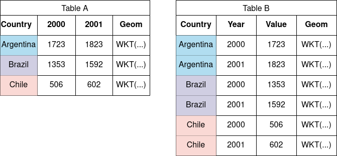
Table A, in that sense, is not tidy since the year variable is not found in its own column but instead it is scattered in two different columns. Table B is a long format with each variable being found in exactly one column. In that sense, each individual row represents exactly one observation, meaning the observation of a specific country in a specific year.
When we structure data in the long format the objects will usually have a larger memory footprint than compared to a wide format. For smaller objects or data types with small memory consumption, this might not pose a serious limitation to the workflow. However, geometry information, here indicated as a WKT string, might quickly accumulate a large proportion of the available memory, even more so if the portfolio consists of a high number of complex geometries that are then copied to fit the the long-format requirement. For that reason, this packages uses a nested-list format to hold tables for indicators as single columns within the portfolio. The remainder of this tutorial will show you in more detail how you can work with those R specific data format.
The simple case - single-row indicators
We start by reading a GeoPackage from disk. For the sake of the argument, we split the original single polygon into 9 distinct polygons to simulate a realistic portfolio consisting of multiple assets.
aoi <- read_sf(
  system.file("extdata", "sierra_de_neiba_478140_2.gpkg",
    package = "mapme.biodiversity"
  )
)
aoi <- st_as_sf(st_make_grid(aoi, n = 3))
print(aoi)
#> Simple feature collection with 9 features and 0 fields
#> Geometry type: POLYGON
#> Dimension:     XY
#> Bounding box:  xmin: -71.80933 ymin: 18.57668 xmax: -71.33201 ymax: 18.69931
#> Geodetic CRS:  WGS 84
#>                                x
#> 1 POLYGON ((-71.80933 18.5766...
#> 2 POLYGON ((-71.65022 18.5766...
#> 3 POLYGON ((-71.49111 18.5766...
#> 4 POLYGON ((-71.80933 18.6175...
#> 5 POLYGON ((-71.65022 18.6175...
#> 6 POLYGON ((-71.49111 18.6175...
#> 7 POLYGON ((-71.80933 18.6584...
#> 8 POLYGON ((-71.65022 18.6584...
#> 9 POLYGON ((-71.49111 18.6584...
As a simple example, suppose we interested in extracting the average traveltime to cities between 20,000 and 50,000 inhabitants in our portfolio. As usual, we will have to make available the Nelson et al. resource as well as requesting the calculation of the respective indicator.
outdir <- file.path(tempdir(), "mapme-resources")
dir.create(outdir, showWarnings = FALSE)

mapme_options(
  outdir = outdir,
  verbose = FALSE
)

aoi <- get_resources(aoi, get_nelson_et_al(ranges = "100k_200k"))
aoi <- calc_indicators(aoi, calc_traveltime(stats = "mean"))
print(aoi)
#> Simple feature collection with 9 features and 2 fields
#> Geometry type: POLYGON
#> Dimension:     XY
#> Bounding box:  xmin: -71.80933 ymin: 18.57668 xmax: -71.33201 ymax: 18.69931
#> Geodetic CRS:  WGS 84
#> # A tibble: 9 × 3
#>   assetid traveltime                                                           x
#>     <int> <list>                                                   <POLYGON [°]>
#> 1       1 <tibble [1 × 4]> ((-71.80933 18.57668, -71.65022 18.57668, -71.65022 …
#> 2       2 <tibble [1 × 4]> ((-71.65022 18.57668, -71.49111 18.57668, -71.49111 …
#> 3       3 <tibble [1 × 4]> ((-71.49111 18.57668, -71.33201 18.57668, -71.33201 …
#> 4       4 <tibble [1 × 4]> ((-71.80933 18.61756, -71.65022 18.61756, -71.65022 …
#> 5       5 <tibble [1 × 4]> ((-71.65022 18.61756, -71.49111 18.61756, -71.49111 …
#> 6       6 <tibble [1 × 4]> ((-71.49111 18.61756, -71.33201 18.61756, -71.33201 …
#> 7       7 <tibble [1 × 4]> ((-71.80933 18.65844, -71.65022 18.65844, -71.65022 …
#> 8       8 <tibble [1 × 4]> ((-71.65022 18.65844, -71.49111 18.65844, -71.49111 …
#> 9       9 <tibble [1 × 4]> ((-71.49111 18.65844, -71.33201 18.65844, -71.33201 …
As we can observe from the output, a new column was added to the
sf object. It is called traveltime and is of
type list indicating that it represents a nested-list
column. What that means is that we are able to maintain the rectangular
shape of our original data (e.g. one polygon per row), while supporting
arbitrarily shaped outputs for indicators. Let’s observe how the
traveltime indicator looks like in this instance:
print(aoi$traveltime[[1]])
#> # A tibble: 1 × 4
#>   datetime            variable                  unit    value
#>   <dttm>              <chr>                     <chr>   <dbl>
#> 1 2015-01-01 00:00:00 100k_200k_traveltime_mean minutes  206.
From the syntax above, you can see how you can access a single object
within the nested list column (e.g. by using the list accessor
[[). In this case, the shape of the traveltime
indicator is a single-row and two-column tibble with the average minutes
and the distance category as its value. We can now use either of two
functions to transform the portfolio to long or wide formats:
portfolio_long(aoi)
#> Simple feature collection with 9 features and 6 fields
#> Geometry type: POLYGON
#> Dimension: XY
#> Bounding box: xmin: -71.80933 ymin: 18.57668 xmax: -71.33201 ymax: 18.69931
#> Geodetic CRS: WGS 84
#> # A tibble: 9 × 7
#> assetid indicator datetime variable unit value
#> <int> <chr> <dttm> <chr> <chr> <dbl>
#> 1 1 traveltime 2015-01-01 00:00:00 100k_200k_traveltime_mean minutes 206.
#> 2 2 traveltime 2015-01-01 00:00:00 100k_200k_traveltime_mean minutes 273.
#> 3 3 traveltime 2015-01-01 00:00:00 100k_200k_traveltime_mean minutes 283.
#> 4 4 traveltime 2015-01-01 00:00:00 100k_200k_traveltime_mean minutes 237.
#> 5 5 traveltime 2015-01-01 00:00:00 100k_200k_traveltime_mean minutes 308.
#> 6 6 traveltime 2015-01-01 00:00:00 100k_200k_traveltime_mean minutes 265.
#> 7 7 traveltime 2015-01-01 00:00:00 100k_200k_traveltime_mean minutes 287.
#> 8 8 traveltime 2015-01-01 00:00:00 100k_200k_traveltime_mean minutes 299.
#> 9 9 traveltime 2015-01-01 00:00:00 100k_200k_traveltime_mean minutes 235.
#> # ℹ 1 more variable: x <POLYGON [°]>
portfolio_wide(aoi)
#> Simple feature collection with 9 features and 2 fields
#> Geometry type: POLYGON
#> Dimension: XY
#> Bounding box: xmin: -71.80933 ymin: 18.57668 xmax: -71.33201 ymax: 18.69931
#> Geodetic CRS: WGS 84
#> # A tibble: 9 × 3
#> assetid traveltime_2015-01-01_100k_200k_traveltime…¹ x
#> <dbl> <dbl> <POLYGON [°]>
#> 1 1 206. ((-71.80933 18.57668, -7…
#> 2 2 273. ((-71.65022 18.57668, -7…
#> 3 3 283. ((-71.49111 18.57668, -7…
#> 4 4 237. ((-71.80933 18.61756, -7…
#> 5 5 308. ((-71.65022 18.61756, -7…
#> 6 6 265. ((-71.49111 18.61756, -7…
#> 7 7 287. ((-71.80933 18.65844, -7…
#> 8 8 299. ((-71.65022 18.65844, -7…
#> 9 9 235. ((-71.49111 18.65844, -7…
#> # ℹ abbreviated name:
#> # ¹`traveltime_2015-01-01_100k_200k_traveltime_mean_minutes`Both function will, by default, automatically detect nested-list
columns and change the data layout. In this case, the result still has 9
rows just like the original data frame because the indicator
traveltime consisted of just a single row per asset.
We could serialize the object to disk in either format by calling
write_portfolio() with the respective format
argument:
dsn_long <- tempfile(fileext = ".gpkg")
dsn_wide <- tempfile(fileext = ".gpkg")
write_portfolio(aoi, dsn_long, format = "long", quiet = TRUE)
write_portfolio(aoi, dsn_wide, format = "wide", quiet = TRUE)
The harder case - indicators with multi-row output
Let’s continue to query an indicator which has a multi-row output, i.e. precipitation statistics from WorldClim.
aoi <- get_resources(aoi, get_worldclim_precipitation(years = 2018))
aoi <- calc_indicators(aoi, calc_precipitation_wc(stats = "mean"))
print(aoi)
#> Simple feature collection with 9 features and 3 fields
#> Geometry type: POLYGON
#> Dimension:     XY
#> Bounding box:  xmin: -71.80933 ymin: 18.57668 xmax: -71.33201 ymax: 18.69931
#> Geodetic CRS:  WGS 84
#> # A tibble: 9 × 4
#>   assetid traveltime       precipitation_wc                                    x
#>     <int> <list>           <list>                                  <POLYGON [°]>
#> 1       1 <tibble [1 × 4]> <tibble [12 × 4]> ((-71.80933 18.57668, -71.65022 18…
#> 2       2 <tibble [1 × 4]> <tibble [12 × 4]> ((-71.65022 18.57668, -71.49111 18…
#> 3       3 <tibble [1 × 4]> <tibble [12 × 4]> ((-71.49111 18.57668, -71.33201 18…
#> 4       4 <tibble [1 × 4]> <tibble [12 × 4]> ((-71.80933 18.61756, -71.65022 18…
#> 5       5 <tibble [1 × 4]> <tibble [12 × 4]> ((-71.65022 18.61756, -71.49111 18…
#> 6       6 <tibble [1 × 4]> <tibble [12 × 4]> ((-71.49111 18.61756, -71.33201 18…
#> 7       7 <tibble [1 × 4]> <tibble [12 × 4]> ((-71.80933 18.65844, -71.65022 18…
#> 8       8 <tibble [1 × 4]> <tibble [12 × 4]> ((-71.65022 18.65844, -71.49111 18…
#> 9       9 <tibble [1 × 4]> <tibble [12 × 4]> ((-71.49111 18.65844, -71.33201 18…
We see that in addition to the traveltime indicator, we
now obtained an additional nested-list column called
precipitation_wc. Note, however, the differences in the
shape of the indicator tibble when we take a closer look for a specific
asset:
print(aoi$precipitation_wc[[1]])
#> # A tibble: 12 × 4
#>    datetime            variable            unit  value
#>    <dttm>              <chr>               <chr> <dbl>
#>  1 2018-01-01 00:00:00 worldclim_prec_mean mm      NaN
#>  2 2018-02-01 00:00:00 worldclim_prec_mean mm      NaN
#>  3 2018-03-01 00:00:00 worldclim_prec_mean mm      NaN
#>  4 2018-04-01 00:00:00 worldclim_prec_mean mm      NaN
#>  5 2018-05-01 00:00:00 worldclim_prec_mean mm      NaN
#>  6 2018-06-01 00:00:00 worldclim_prec_mean mm      NaN
#>  7 2018-07-01 00:00:00 worldclim_prec_mean mm      NaN
#>  8 2018-08-01 00:00:00 worldclim_prec_mean mm      NaN
#>  9 2018-09-01 00:00:00 worldclim_prec_mean mm      NaN
#> 10 2018-10-01 00:00:00 worldclim_prec_mean mm      NaN
#> 11 2018-11-01 00:00:00 worldclim_prec_mean mm      NaN
#> 12 2018-12-01 00:00:00 worldclim_prec_mean mm      NaN
For a single asset, we obtain a tibble with 12 rows (for each month
in the queried year 2018). Now, let’s have a look at what happens if we
transform this table to long format, this time specifically requesting
to only extract the precipitation_wc indicators:
portfolio_long(aoi, indicators = "precipitation_wc")
#> Simple feature collection with 108 features and 7 fields
#> Geometry type: POLYGON
#> Dimension:     XY
#> Bounding box:  xmin: -71.80933 ymin: 18.57668 xmax: -71.33201 ymax: 18.69931
#> Geodetic CRS:  WGS 84
#> # A tibble: 108 × 8
#>    assetid traveltime       indicator   datetime            variable unit  value
#>      <int> <list>           <chr>       <dttm>              <chr>    <chr> <dbl>
#>  1       1 <tibble [1 × 4]> precipitat… 2018-01-01 00:00:00 worldcl… mm      NaN
#>  2       1 <tibble [1 × 4]> precipitat… 2018-02-01 00:00:00 worldcl… mm      NaN
#>  3       1 <tibble [1 × 4]> precipitat… 2018-03-01 00:00:00 worldcl… mm      NaN
#>  4       1 <tibble [1 × 4]> precipitat… 2018-04-01 00:00:00 worldcl… mm      NaN
#>  5       1 <tibble [1 × 4]> precipitat… 2018-05-01 00:00:00 worldcl… mm      NaN
#>  6       1 <tibble [1 × 4]> precipitat… 2018-06-01 00:00:00 worldcl… mm      NaN
#>  7       1 <tibble [1 × 4]> precipitat… 2018-07-01 00:00:00 worldcl… mm      NaN
#>  8       1 <tibble [1 × 4]> precipitat… 2018-08-01 00:00:00 worldcl… mm      NaN
#>  9       1 <tibble [1 × 4]> precipitat… 2018-09-01 00:00:00 worldcl… mm      NaN
#> 10       1 <tibble [1 × 4]> precipitat… 2018-10-01 00:00:00 worldcl… mm      NaN
#> # ℹ 98 more rows
#> # ℹ 1 more variable: x <POLYGON [°]>
Instead of 9 rows, we get a tibble with 108 rows (9 assets * 12), with the metadata for each asset with the geometry column and other identifying values being repeated 12 times each. For very large portfolios, this data layout might be very memory intensive. In these cases it might be more favourable to transform the portfolio to a wide layout.
portfolio_wide(aoi, indicators = "precipitation_wc")
#> Simple feature collection with 9 features and 14 fields
#> Geometry type: POLYGON
#> Dimension: XY
#> Bounding box: xmin: -71.80933 ymin: 18.57668 xmax: -71.33201 ymax: 18.69931
#> Geodetic CRS: WGS 84
#> # A tibble: 9 × 15
#> assetid traveltime precipitation_wc_2018-01-01_…¹ precipitation_wc_201…²
#> <dbl> <list> <dbl> <dbl>
#> 1 1 <tibble [1 × 4]> NaN NaN
#> 2 2 <tibble [1 × 4]> 29 27.2
#> 3 3 <tibble [1 × 4]> 24.4 24.0
#> 4 4 <tibble [1 × 4]> 31.9 28.0
#> 5 5 <tibble [1 × 4]> 28.5 28.2
#> 6 6 <tibble [1 × 4]> 18.9 21.1
#> 7 7 <tibble [1 × 4]> 24.4 24.2
#> 8 8 <tibble [1 × 4]> 19.3 21.0
#> 9 9 <tibble [1 × 4]> NaN NaN
#> # ℹ abbreviated names: ¹`precipitation_wc_2018-01-01_worldclim_prec_mean_mm`,
#> # ²`precipitation_wc_2018-02-01_worldclim_prec_mean_mm`
#> # ℹ 11 more variables:
#> # `precipitation_wc_2018-03-01_worldclim_prec_mean_mm` <dbl>,
#> # `precipitation_wc_2018-04-01_worldclim_prec_mean_mm` <dbl>,
#> # `precipitation_wc_2018-05-01_worldclim_prec_mean_mm` <dbl>,
#> # `precipitation_wc_2018-06-01_worldclim_prec_mean_mm` <dbl>, …From the example output above we see that in this case, we obtain a resulting object with 9 rows only. The indicator data is now found in the respective columns which are named according to this schema:
<indicator-name>_<datetime>_<variable>_<unit>
with the values being found in the rows for each unique combination of this pattern.
Note, that the traveltime still is represented as a
nested-list column. When serializing to disk, all present indicators are
going to extracted in order to be able to serialize to spatial data
formats. If it is not desired to include certain indicators you will
have to subset the portfolio as indicated in the following code
block:
dsn <- tempfile(fileext = ".gpkg")
write_portfolio(select(aoi, traveltime), dsn, quiet = TRUE)