Introduction
In the following we will demonstrate an idealized workflow based on a subset of the Global Forest Watch (GFW) data set that is delivered together with this package. You can follow along the code snippets below to reproduce the results. Please note that to reduce the time it takes to process this vignette, we will not download any resources from the internet. In a real use case, thus processing time might substantially increase because resources have to be downloaded and real portfolios might be larger than the one created in this example.
This vignette assumes that you have already followed the steps in Installation and have familiarized yourself with the terminology used in the package. If you are unfamiliar with the terminology used here, please head over to the Terminology article to learn about the most important concepts.
The idealized workflow for using mapme.biodiversity consists of the following steps:
- prepare your sf-object containing only geometries of type
'POLYGON'or'MULTIPOLYGON' - decide which indicator(s) you wish to calculate and make the required resource(s) available
- conduct your indicator calculation, which adds a nested list column to your portfolio object
- continue your analysis in R or decide to export your results to a spatial data format to use it with other geospatial software
Getting started
First, we will load the mapme.biodiversity and the sf package for handling spatial vector data. For tabular data handling, we will also load the dplyr and tidyr packages. Then, we will read an internal GeoPackage which includes part of the geometry of a protected area in the Dominican Republic from the WDPA database.
library(mapme.biodiversity)
library(sf)
library(dplyr)
library(tidyr)

aoi_path <- system.file("extdata", "gfw_sample.gpkg", package = "mapme.biodiversity")
aoi <- st_read(aoi_path, quiet = TRUE)
aoi
#> Simple feature collection with 1 feature and 0 fields
#> Geometry type: POLYGON
#> Dimension:     XY
#> Bounding box:  xmin: -71.73773 ymin: 18.63179 xmax: -71.69 ymax: 18.68691
#> Geodetic CRS:  WGS 84
#>                             geom
#> 1 POLYGON ((-71.73417 18.6435...
Setting standard option
We use the mapme_options() function and set some
arguments, such as the output directory, that are important to govern
the subsequent processing. For this, we create a temporary directory.
Internally, to save time on downloading when building this vignette, we
copied already existing files to that output location (code not shown
here).
outdir <- file.path(tempdir(), "mapme-resources")
dir.create(outdir, showWarnings = FALSE)

mapme_options(
  outdir = outdir,
  verbose = TRUE
)
The outdir argument points towards a directory on the
local file system of your machine. All downloaded resources will be
written to respective directories nested within outdir.
Once you request a specific resource for your portfolio, only those
files will be downloaded that are missing to match its spatio-temporal
extent. This behaviour is beneficial, e.g. in case you share the
outdir between different projects to ensure that only
resources matching your current portfolio are returned.
The verbose logical controls whether or not the package
will print informative messages during the calculations. Note, that even
if set to FALSE, the package will inform users about any
potential errors or warnings.
Getting the right resources
You can check which indicators are available via the
available_indicators() function:
available_indicators()
#> # A tibble: 40 × 3
#>    name                          description                           resources
#>    <chr>                         <chr>                                 <list>
#>  1 biodiversity_intactness_index Averaged biodiversity intactness ind… <tibble>
#>  2 biome                         Areal statistics of biomes from TEOW  <tibble>
#>  3 burned_area                   Monthly burned area detected by MODI… <tibble>
#>  4 deforestation_drivers         Areal statistics of deforestation dr… <tibble>
#>  5 drought_indicator             Relative wetness statistics based on… <tibble>
#>  6 ecoregion                     Areal statistics of ecoregions based… <tibble>
#>  7 elevation                     Statistics of elevation based on NAS… <tibble>
#>  8 exposed_population_acled      Number of people exposed to conflict… <tibble>
#>  9 exposed_population_ucdp       Number of people exposed to conflict… <tibble>
#> 10 fatalities_acled              Number of fatalities by event type b… <tibble>
#> # ℹ 30 more rows
available_indicators("treecover_area")
#> # A tibble: 1 × 3
#>   name           description                  resources
#>   <chr>          <chr>                        <list>
#> 1 treecover_area Area of forest cover by year <tibble [2 × 5]>
Say, we are interested in the treecover_area indicator.
We can learn more about this indicator and its required resources by
using either of the commands below or, if you are viewing the online
version, head over to the treecover_area
documentation.
?treecover_area
help(treecover_area)
By inspecting the help page we learned that this indicator requires
the gfw_treecover and gfw_lossyear resources
and it requires to specify three extra arguments: the years for which to
calculate treecover, the minimum size of patches to be considered as
forest and the minimum canopy coverage of a single pixel to be
considered as forested.
With that information at hand, we can start to retrieve the required
resource. We can learn about all available resources using the
available_resources() function:
available_resources()
#> # A tibble: 35 × 5
#>    name                          description                licence source type
#>    <chr>                         <chr>                      <chr>   <chr>  <chr>
#>  1 accessibility_2000            Accessibility data for th… See JR… https… rast…
#>  2 acled                         Armed Conflict Location &… Visit … Visit… vect…
#>  3 biodiversity_intactness_index Biodiversity Intactness I… CC-BY-… https… rast…
#>  4 chelsa                        Climatologies at High res… Unknow… https… rast…
#>  5 chirps                        Climate Hazards Group Inf… CC - u… https… rast…
#>  6 esalandcover                  Copernicus Land Monitorin… CC-BY … https… rast…
#>  7 fritz_et_al                   Drivers of deforestation … CC-BY … https… rast…
#>  8 gfw_emissions                 Global Forest Watch - CO2… CC-BY … https… rast…
#>  9 gfw_lossyear                  Global Forest Watch - Yea… CC-BY … https… rast…
#> 10 gfw_treecover                 Global Forest Watch - Per… CC-BY … https… rast…
#> # ℹ 25 more rows
available_resources("gfw_treecover")
#> # A tibble: 1 × 5
#>   name          description                                 licence source type
#>   <chr>         <chr>                                       <chr>   <chr>  <chr>
#> 1 gfw_treecover Global Forest Watch - Percentage of canopy… CC-BY … https… rast…
For the purpose of this vignette, we are going to download both, the
gfw_treecover and gfw_lossyear resources. We
can get more detailed information about a given resource, by using
either of the commands below to open up the help page. If you are
viewing the online version of this documentation, you can simply head
over to the gfw_treecover
resource documentation.
We can now make the required resources available for our portfolio.
We will use a common interface that is used for all resources, called
get_resources(). We have to specify our portfolio object
and supply one or more resource functions with their respective
arguments. This will then download the matching resources to the output
directory specified earlier.
aoi <- get_resources(
  x = aoi,
  get_gfw_treecover(version = "GFC-2023-v1.11"),
  get_gfw_lossyear(version = "GFC-2023-v1.11")
)
Calculate specific indicators
The next step consists of calculating specific indicators. Note that
each indicator requires one or more resources that were made available
via the get_resources() function explained above. You will
have to re-run this function in every new R session, but note that data
that is already available will not be re-downloaded.
Here, we are going to calculate the treecover_area
indicator which is based on the resources from GFW. Since the resources
have been made available in the previous step, we can continue
requesting the calculation of our desired indicator. Note the command
below would issue an error in case a required resource has not been made
available via get_resources() beforehand.
aoi <- calc_indicators(
  aoi,
  calc_treecover_area(years = 2000:2023, min_size = 1, min_cover = 30)
)
Now let’s take a look at the results. In addition to the metadata we
are already familiar with, we see that there is an additional column
called treecover_area which contains a
tibble.
aoi
#> Simple feature collection with 1 feature and 2 fields
#> Geometry type: POLYGON
#> Dimension:     XY
#> Bounding box:  xmin: -71.73773 ymin: 18.63179 xmax: -71.69 ymax: 18.68691
#> Geodetic CRS:  WGS 84
#> # A tibble: 1 × 3
#>   assetid treecover_area                                                    geom
#>     <int> <list>                                                   <POLYGON [°]>
#> 1       1 <tibble [24 × 4]> ((-71.73735 18.64734, -71.71386 18.63179, -71.69 18…
The indicator is represented as a nested-list column in our
sf-object that is named alike the requested indicator. For
our single asset, this column contains a tibble with 24 rows and four
columns. Let’s have a closer look at this object
aoi$treecover_area
#> [[1]]
#> # A tibble: 24 × 4
#> datetime variable unit value
#> <dttm> <chr> <chr> <dbl>
#> 1 2000-01-01 00:00:00 treecover ha 1976.
#> 2 2001-01-01 00:00:00 treecover ha 1976.
#> 3 2002-01-01 00:00:00 treecover ha 1974.
#> 4 2003-01-01 00:00:00 treecover ha 1941.
#> 5 2004-01-01 00:00:00 treecover ha 1931.
#> 6 2005-01-01 00:00:00 treecover ha 1927.
#> 7 2006-01-01 00:00:00 treecover ha 1920.
#> 8 2007-01-01 00:00:00 treecover ha 1909.
#> 9 2008-01-01 00:00:00 treecover ha 1906.
#> 10 2009-01-01 00:00:00 treecover ha 1904.
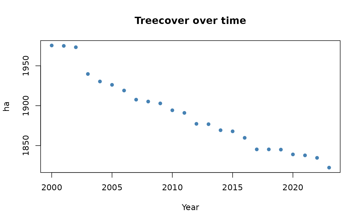
#> # ℹ 14 more rowsThe tibble follows a standard output format, which is the same for
all indicators. Each indicator is represented as a tibble with the four
columns datetime, variable, unit,
and value. In case of the treecover_area
indicator, the variable is called treecover and is
expressed in ha.
Let’s quickly visualize the results:
If you wish to change the layout of an portfolio, you can use
portfolio_long() and portfolio_wide() (see the
respective online
tutorial). Especially for large portfolios, it is usually a good
idea to keep the geometry information in a separated variable to keep
the size of the data object relatively small.
geoms <- st_geometry(aoi)
portfolio_long(aoi, drop_geoms = TRUE)
#> # A tibble: 24 × 6
#>    assetid indicator      datetime            variable  unit  value
#>      <int> <chr>          <dttm>              <chr>     <chr> <dbl>
#>  1       1 treecover_area 2000-01-01 00:00:00 treecover ha    1976.
#>  2       1 treecover_area 2001-01-01 00:00:00 treecover ha    1976.
#>  3       1 treecover_area 2002-01-01 00:00:00 treecover ha    1974.
#>  4       1 treecover_area 2003-01-01 00:00:00 treecover ha    1941.
#>  5       1 treecover_area 2004-01-01 00:00:00 treecover ha    1931.
#>  6       1 treecover_area 2005-01-01 00:00:00 treecover ha    1927.
#>  7       1 treecover_area 2006-01-01 00:00:00 treecover ha    1920.
#>  8       1 treecover_area 2007-01-01 00:00:00 treecover ha    1909.
#>  9       1 treecover_area 2008-01-01 00:00:00 treecover ha    1906.
#> 10       1 treecover_area 2009-01-01 00:00:00 treecover ha    1904.
#> # ℹ 14 more rows
A note on parallel computing
mapme.biodiversity follows the parallel computing
paradigm of the {future}
package. That means that you as a user are in the control if and how you
would like to set up parallel processing. Since
{mapme.biodiversity} v0.9, we apply pre-chunking to all
assets in the portfolio. That means that assets are split up into
components of roughly the size of chunk_size. These
components can than be iterated over in parallel to speed up processing.
Indicator values will be aggregated automatically.
As another example, with the code below one would apply parallel processing of 2 assets, with each having 4 workers available to process chunks, thus requiring a total of 8 available cores on the host machine. Be sure to not request more workers than available on your machine.
library(progressr)

plan(cluster, workers = 2)

with_progress({
  aoi <- calc_indicators(
    aoi,
    calc_treecover_area_and_emissions(
      min_size = 1,
      min_cover = 30
    )
  )
})

plan(sequential) # close child processes
Exporting an portfolio object
You can use the write_portfolio() function to save a
processed portfolio object to disk as a GeoPackage. This
allows sharing your data with contributors who might not be using R, but
any other geospatial software. Simply point towards a non-existing file
on your local disk to write the portfolio. You can use
read_portfolio() to read back a GeoPackage written in such
a way into R:
dsn <- tempfile(fileext = ".gpkg")
write_portfolio(x = aoi, dsn = dsn, quiet = TRUE)
from_disk <- read_portfolio(dsn, quiet = TRUE)
from_disk
#> Simple feature collection with 1 feature and 2 fields
#> Geometry type: POLYGON
#> Dimension:     XY
#> Bounding box:  xmin: -71.73773 ymin: 18.63179 xmax: -71.69 ymax: 18.68691
#> Geodetic CRS:  WGS 84
#> # A tibble: 1 × 3
#>   assetid treecover_area                                                    geom
#>     <int> <list>                                                   <POLYGON [°]>
#> 1       1 <tibble [24 × 4]> ((-71.73735 18.64734, -71.71386 18.63179, -71.69 18…
#> [1] TRUE